I was always curious about how the images of black holes came to be. I knew how to derive the Schwarzschild metric and how to solve the geodesic equations from the General Relativity lectures I took. Yet I never tried creating the full image.

I set out to build a raytracer (gr_raytracer) that is as generic as possible: new geometries can be added and geodesic equations can be solved in different ways, while the overall raytracing logic stays the same. At its core, a component takes a ray with a 4-position ($x^\mu$) and a 4-momentum ($p^\mu$) and integrates it into a trajectory (a sequence of positions and momenta). This integration step is the shared foundation across all geometries.

Those rays are then checked for intersections with objects and assigned a color.

But let us first look at what makes a raytracer in curved spacetime special.

Raytracing

One big difference is that in Euclidean geometry it is simple to define a ray as

\[\mathbf{x}(t) = \mathbf{x}_0 + t\, \mathbf{d}\,.\]

Here, the parameter $t$ is a simple curve parameter. In the Euclidean case, this simple form allows closed-form intersection tests with various objects like triangles or spheres. We could just set up a ray belonging to a pixel on the camera and check for all possible intersections. More complex topics like reflections and lighting are not covered here, as the General Relativity raytracer does not handle them. It just checks if it hit an object or escaped to infinity and then computes a color from some internal data of the object, like the temperature or a texture.

In General Relativity, on the other hand, we integrate with respect to an affine parameter $\lambda$ (since we are dealing with photons, these are null geodesics).

The basic concept is shown in Figure 1, where we have a pinhole camera that collects light. To compute this, the actual algorithm shoots rays from the pinhole camera through a screen until they reach an object. As described above, light sources are ignored in this case, assuming the objects are self-illuminating. Each ray is assigned a pixel on the screen based on where it crosses the corresponding part of the image plane.

Figure 1: Raytracer Euclidean

With a raytracer in a curved space, this will look different. Let’s look at an example with a Schwarzschild black hole. Note that these are not correct trajectories but just an illustration to show the principle.

Figure 2: Black Hole Raytracer Illustration

These trajectories are given by the geodesic equations:

\[\frac{d^2x^\mu}{d\lambda^2} + \Gamma^\mu_{\alpha\beta} \frac{dx^\alpha}{d\lambda} \frac{dx^\beta}{d\lambda} = 0\]

As mentioned, more details about them will come in later posts. This also means we cannot just directly compute intersections via simple algebraic formulas, but must instead step along the geodesic, checking for intersections at each discrete interval. For this, a numerical integration method has to be used. In this case, it is an adaptive Runge-Kutta-Fehlberg (RKF45) method.

The Pipeline

The renderer creates sRGB and HDR images. It uses rayon, a Rust parallelism library, to parallelize the computation. Each ray goes through the integration stage. The resulting trajectory is then analyzed for intersections with various object types, from which a final color is assigned.

The integration stage accepts a geometry definition, which provides the geodesic equations to be integrated. More details about that will come in later posts.

Figure 3: Raytracer Architecture

Example Result

The final result of a render of a near-extremal Kerr black hole with an accretion disk looks like this:

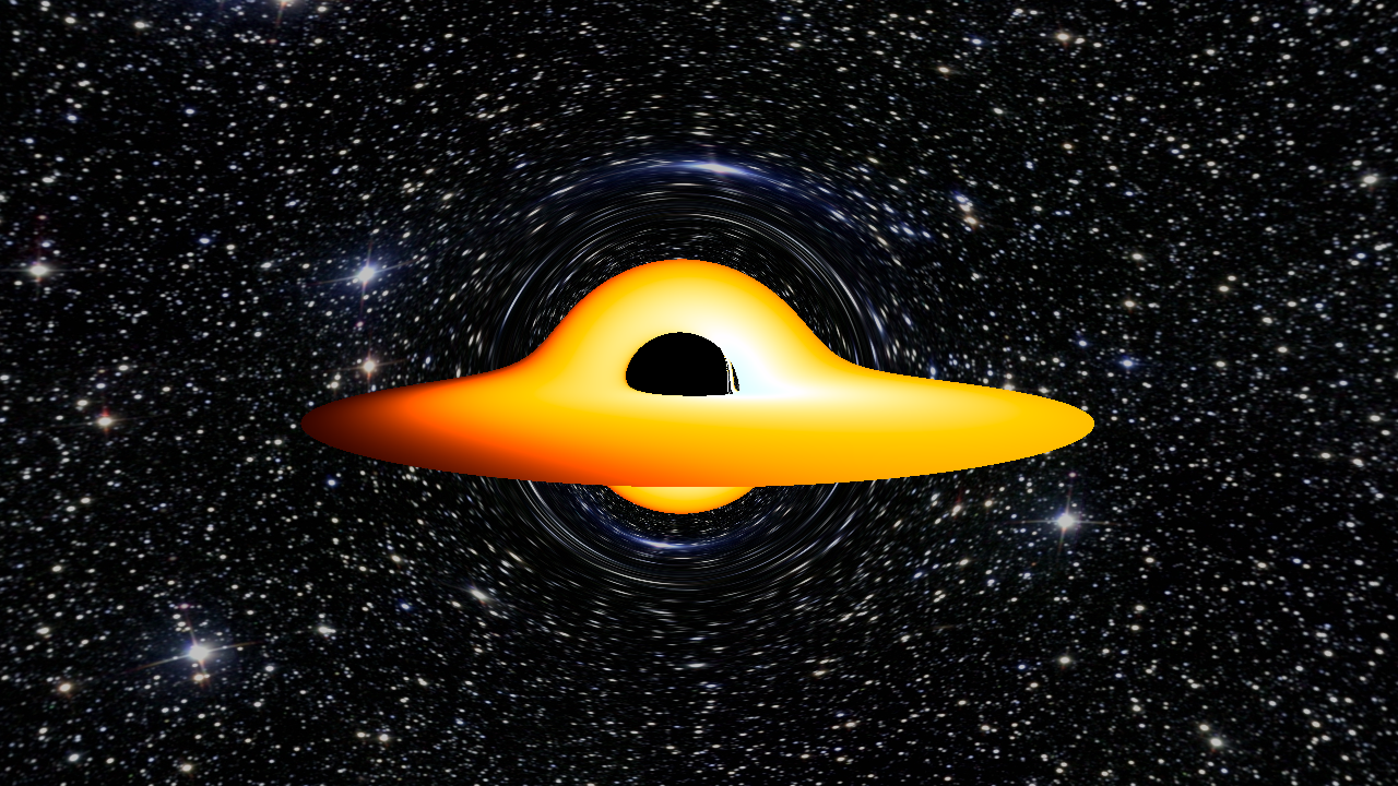
Figure 4: Render of a Kerr Black Hole

The visible distortion of the accretion disk, where the part behind the black hole appears to be bent up and over it, is a direct visual consequence of gravitational lensing.

The background image is Messier 25 from Wikimedia Commons.

The next post digs into why straight lines aren’t so straightforward in curved coordinates and how that motivates the geodesic equation: Straight Lines in Curved Coordinates.